HSIM v3
The HARMONI Simulator
HARMONI has a dedicated tool for performing quantitative simulations of HARMONI observations. The HARMONI simulation pipeline was developed at Oxford (Zieleniewski et al. 2015b), and used to develop several key science cases, as part of the design and development of the HARMONI integral field spectrograph. The tool has since been enhanced and entirely re-written by M. Pereira-Santaella.
The goal is to be able to simulate the performance of the instrument folding in detailed parameters including the ELT AO performance, atmospheric effects and realistic detector statistics. This webpage will be regularly updated as the simulator pipeline evolves and improves.
System Requirements
The pipeline is written in Python3. It should run on any OS as long as the relevant Python libraries are installed (see below). We have tested it on Mac OSX and Linux (Ubuntu 18.04). It is possible to run on Windows, but we have done little testing.
The required Python modules are:
- astropy 3.2.1 - https://www.astropy.org/
- numpy 1.17.0 - https://www.scipy.org/install.html
- scipy 1.3.1 - https://www.scipy.org/install.html
- matplotlib 3.1.1 - https://matplotlib.org/
- photutils 0.7 - https://photutils.readthedocs.io/en/stable//
>>> import numpy
>>> import scipy
>>> import astropy
>>> import photutils
>>> import matplotlib
There should be no errors!
Input Datacubes
The pipeline takes an input FITS file datacube containing spatial and spectral information about the astrophysical source of interest. The format should be an (x, y, λ) datacube with each pixel containing the value of flux per sq. arcsec (e.g. erg/s/cm^2/μm/arcsec^2 or MJy/sr). The FITS datacube needs to have the following headers:
- NAXIS1, NAXIS2, NAXIS3 - Size of the x, y, and wavelength axes respectively.
- CTYPE1, CTYPE2, CTYPE3 - Axis type. Accepted values: [x, y, wavelength] or [RA, DEC, wavelength].
- CUNIT1, CUNIT2 - Units for the spatial axes. Accepted values: any angular unit supported by astropy e.g. mas, arcsec.
- CUNIT3 - Units for the spectral axis. Accepted values: any length unit supported by astropy e.g., angstrom, AA, nm, micron.
- CDELT1, CDELT2, CDELT3 - Sampling for each axis in units given by CUNIT1/2/3 headers.
- CRVAL3 - Value of array element given by CRPIX3 in units of CUNIT3.
- CRPIX3 - Denotes the array element for CRVAL3. Should be set to 1 so CRVAL3 denotes first wavelength value.
- BUNIT - Flux units for each element in datacube. Accepted values: any surface spectral flux den- sity unit supported by astropy e.g. erg/s/cm2/um/arcsec2, MJy/sr.
- SPECRES - Spectral resolution element FWHM in units of CUNIT3.
Input Datacube Generator (CUBEGEN)
A simple input data cube generation interface (CUBEGEN) has been created to help with this stage. It has been developed by Simon Zieleniewski based on work by Nicholas Zieleniewski and Sarah Kendrew.The source code can be found HERE.
CUBEGEN allows the user to generate input data cubes for a range of template spectra, as well as user-uploaded files, for both point sources or extended objects (Sersic profiles). The code is still in *beta* stage but has undergone moderate testing.
HSIM Input Parameters
The simulation pipeline allows for various observing parameters. These are listed in order as follows:- Input cube (incl. path)
- Exposure time [s] (ESO header DIT)
- Number of exposures (ESO header NINT)
- Grating: one of [V+R, Iz+J, H+K, Iz, J, H, K, z-high, J-short, J-long, H-high, K-short, K-long]
- Spaxel scale in mas: one of [4x4, 10x10, 20x20, 30x60]
- Zenith seeing: Atmospheric seeing FWHM in arcsec. Available values are [0.43, 0.57, 0.64, 0.72, 1.04]
- Airmass (average value during observation): Available values are [1.1, 1.3, 1.5, 2.0], which correspond to zenith angles of 25°, 40°, 48° and 60° respectively.
- Moon illumination: Fraction of the moon that is illuminated at the time of observation. Available values are [0, 0.5, 1.0,]
- Residual tip-tilt jitter in mas: The generated PSF are jitter-free, and a realistic value for the residual tip-tilt jitter needs to be specified, depending on AO mode. Typical values are σ = 2 mas for SCAO, and σ = 3 mas for LTAO. It is possible to define different jitter values for the two axes (e.g. 2x4)
- Telescope (site) temperature in K. Typical value is 280 K. This is used to calculate the telescope and instrument background.
- ADR on/off: Indicates whether correction for atmospheric differential refraction, as would be performed by the pipeline, is simulated. Available values are True, False, with True implying that the ADR is compensated in the output data cube.
- AO mode: Available values are LTAO, SCAO, noAO, Airy, filename.fits. Airy uses the diffraction limit of the ELT for the PSF. If a filename.fits is specified, it is assumed to be a user-defined PSF with 1 mas sampling, and the same PSF is used for all wavelength channels.
- Detector systematics: Indicates whether the detector systematics are simulated. Available values are True, False.
Simulation Procedure
HSIM3 adopts a "follow-the-photons" philosophy, with the sky, telescope, instrument and detector effects applied in order.
The AO PSF is generated for each wavelength of the cube from a WFE map, which is itself generated from the Power Spectral Density (PSD) of the AO system. Subsequently, the residual tip-tilt jitter is added as a Gaussian with the user-defined σ. It is recommended that the input cube has 1, 2, 3 or 3 mas sampling, for the four HARMONI spaxel scales.
If the input spectral resolution (denoted by the SPECRES header) is finer than the chosen output, the cube is convolved with the corresponding Gaussian line spread function to yield an output at the instrument's resolution. It is recommended to provide an input cube with a factor of 2 better spectral resolution (and Nyquist or better sampling) than the R of the chosen grating.
The effect of atmospheric differential refraction is then added to the datacube, along the longest spatial axis and relative to the central wavelength channel. The ADR model is developed from Kendrew et al. (2008).The datacube is rebinned to the chosen output spaxel scale. Throughput and background cubes are generated using specific models for sky background and transmission (ESO Skycalc), telescope throughput and emission, instrument throughput, and detector QE. Lastly, random and systematic noise is added.
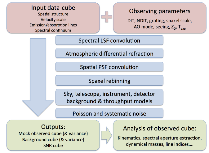
Outputs
The outputs have the basename of the the input cube, with the following suffixes:- _observed_obj_plus_back.fits This is the observed cube representing a mock observation, taking into account the photon noise, read noise, dark current, and cross-talk.
- _reduced.fits This represents the result of an ON-OFF nodding pair, as a simulated "blank sky" observation of equal exposure time is subtracted from the _observed_obj_plus_back.fits data cube.
- _std.fits This cube holds the standard deviation of the total noise for each pixel, including object, sky, dark current and read noise contributions. The noise refers to the observed cube (not reduced cube).
- _reduced_SNR.fits Signal-to-noise ratio of the reduced data cube per pixel.
There are several other outputs, details of which may be found in the manual. The output "observed" cubes represent the result of a perfect data reduction process and are ready to be analysed.